
scSidekick - Co-expression Analysis
16_coexpression.RmdOverview
Three functions cover the co-expression workflow end-to-end:
-
CorrelateGene()- correlate one gene of interest against every other gene, within each cell type, at single-cell, pseudobulk, or group-average resolution. -
PlotCorrelation()- visualize the results as per-cell-type volcano-style plots (r vs. -log10 adjusted p-value). -
SplitByGene()- label each cell as high / low (or expressed / zero) based on a gene’s expression, per cell type. Feeds directly intoRunGSEA_pseudobulk()orFindMarkers().
#for this we will load an object with multiple donors/samples
#InstallData("panc8")
data("panc8")
panc8 <- UpdateSeuratObject(panc8)
panc8 <- NormalizeData(panc8, verbose = FALSE)
panc8$donor=panc8$orig.ident
panc8 <- PrepObject(panc8,
  variables   = c("donor", "celltype"),
  group.by    = "celltype",
  object_name = "panc8")
1. CorrelateGene() - single-cell level
The default level = "sc" computes Spearman correlation
across individual cells within each cell type. Only genes expressed in
at least min_pct% of cells in a given cell type are tested
(expressed_only = TRUE by default).
cor_sc <- CorrelateGene(panc8,
  gene     = "STAT1",
  group.by = "celltype",
  level    = "sc")

head(cor_sc)
## gene cell_type r p padj n goi level
## 1 NME2 acinar -0.3079248 2.033663e-18 2.327934e-14 772 STAT1 sc
## 2 LOC100506281 acinar -0.2992826 1.935724e-17 1.107912e-13 772 STAT1 sc
## 3 MAN1B1 acinar -0.2945833 6.386592e-17 1.982662e-13 772 STAT1 sc
## 4 TAAR5 acinar -0.2942597 6.928145e-17 1.982662e-13 772 STAT1 sc
## 5 EIF4EBP3 acinar -0.2860819 5.236258e-16 1.192260e-12 772 STAT1 sc
## 6 A2M acinar -0.2853201 6.300764e-16 1.192260e-12 772 STAT1 sc
## method
## 1 spearman
## 2 spearman
## 3 spearman
## 4 spearman
## 5 spearman
## 6 spearmanEach row is one gene in one cell type. Key columns:
| Column | Description |
|---|---|
gene |
Correlated gene |
cell_type |
Cell-type group |
r |
Spearman (or Pearson) correlation with the gene of interest |
p |
Raw p-value |
padj |
BH-adjusted p-value |
n |
Number of cells tested |
goi |
Gene of interest |
level |
Resolution used ("sc", "pseudobulk", or
"group") |
2. PlotCorrelation() - visualize results
PlotCorrelation() draws one panel per cell type showing
the top n_pos positively and top n_neg
negatively correlated genes. Significant genes
(padj < padj_cutoff) are colored; the top
label_n in each direction are labeled. Panels are assembled
with patchwork::wrap_plots().
PlotCorrelation(cor_sc,
  n_pos       = 20,
  n_neg       = 20,
  label_n     = 5,
  padj_cutoff = 0.05,
  r_cutoff    = 0.3,     # draws ±0.3 dotted reference lines
  ncol        = 4)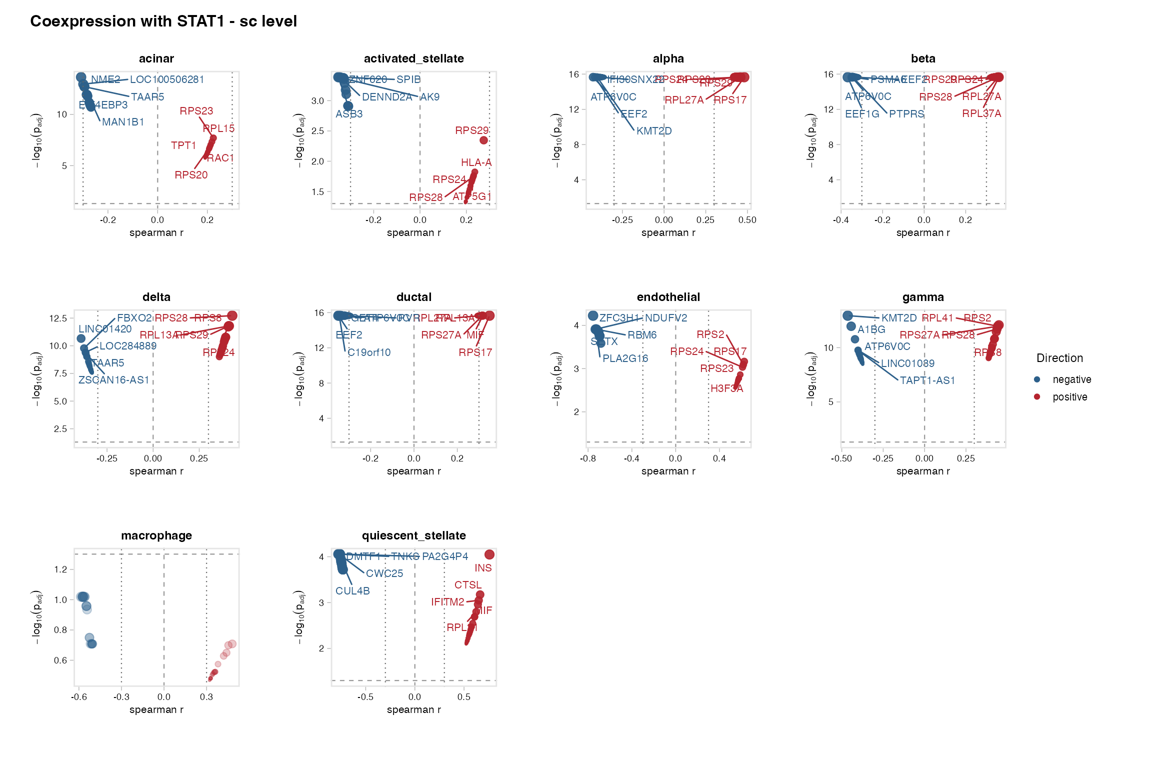
Restrict to specific cell types with cell.type:
PlotCorrelation(cor_sc,
  cell.type = c("acinar", "ductal"),
  n_pos     = 15,
  n_neg     = 15,
  label_n   = 6)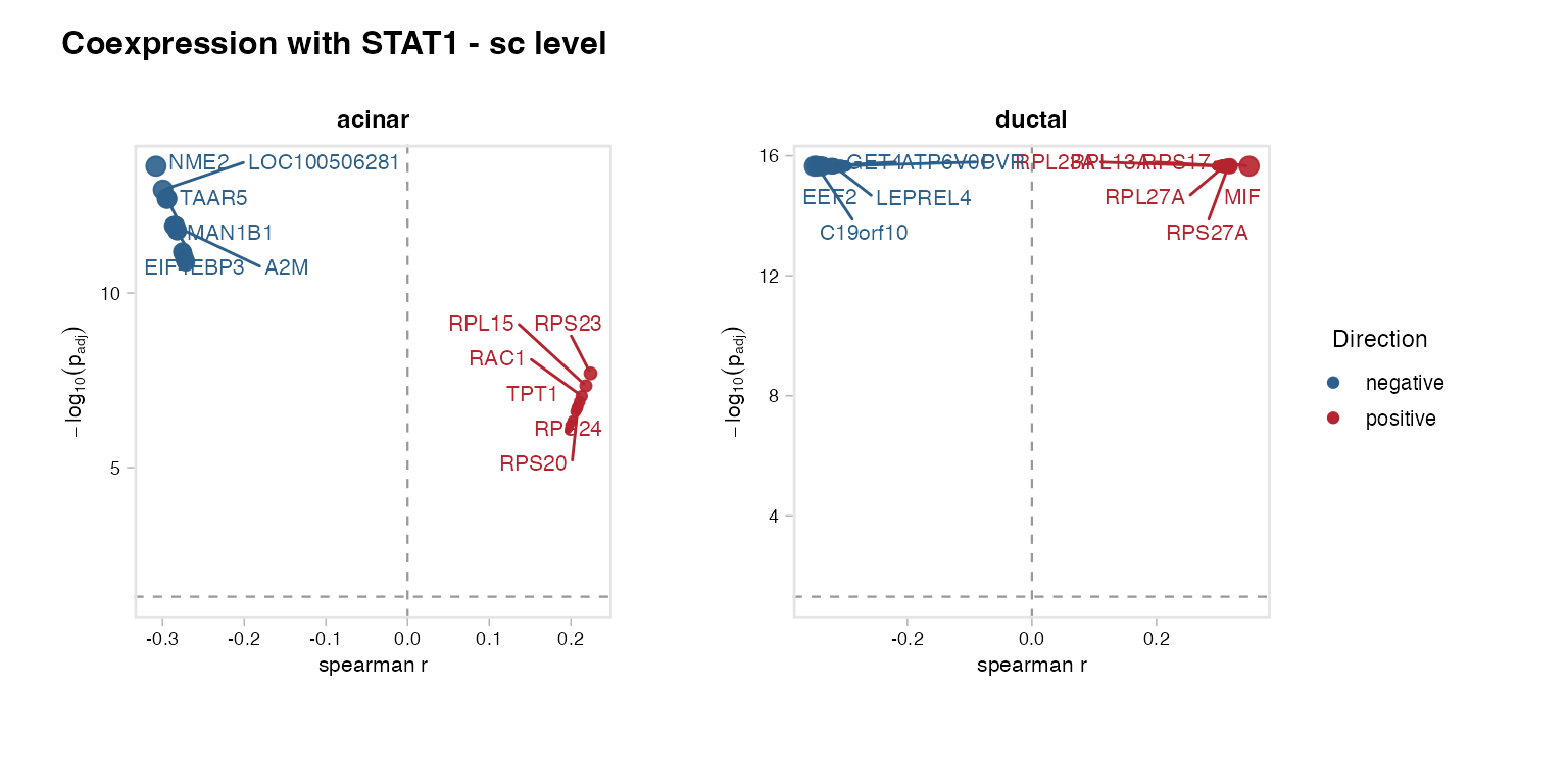
Save to PDF (a .legend sidecar is written
automatically). width/height override the
auto-calculated PDF size, and timestamp = TRUE appends a
_YYYYMMDD-HHMMSS stamp to the saved file name so repeated
runs are versioned instead of overwritten:
PlotCorrelation(cor_sc,
  n_pos      = 20,
  n_neg      = 20,
  output_dir = "./Figures",
  file_name  = "STAT1_coexpression",
  timestamp  = TRUE)
3. CorrelateGene() - pseudobulk level
For multi-donor datasets, pseudobulk correlation
(level = "pseudobulk") aggregates counts to the donor x
cell-type level first. This removes within-donor cell-count inflation
and is more appropriate for multi-sample comparisons. Requires
sample.by.
cor_pb <- CorrelateGene(panc8,
  gene       = "STAT1",
  group.by   = "celltype",
  level      = "pseudobulk",
  sample.by  = "donor",
  min_donors = 3)
Group-average level
level = "group" averages expression within each
combination of cell type and condition.by, then correlates
across those group-level averages. Useful when donors are few but groups
are many (e.g. comparing many cell-type x timepoint combinations).
cor_grp <- CorrelateGene(panc8,
  gene         = "STAT1",
  group.by     = "celltype",
  level        = "sc",
  condition.by = "donor",
  min_groups   = 3)

head(cor_grp)
## gene cell_type r p padj n goi level
## 1 NME2 acinar -0.3079248 2.033663e-18 2.327934e-14 772 STAT1 sc
## 2 LOC100506281 acinar -0.2992826 1.935724e-17 1.107912e-13 772 STAT1 sc
## 3 MAN1B1 acinar -0.2945833 6.386592e-17 1.982662e-13 772 STAT1 sc
## 4 TAAR5 acinar -0.2942597 6.928145e-17 1.982662e-13 772 STAT1 sc
## 5 EIF4EBP3 acinar -0.2860819 5.236258e-16 1.192260e-12 772 STAT1 sc
## 6 A2M acinar -0.2853201 6.300764e-16 1.192260e-12 772 STAT1 sc
## method
## 1 spearman
## 2 spearman
## 3 spearman
## 4 spearman
## 5 spearman
## 6 spearman4. Stratified analysis with compare.by
Pass compare.by to run the correlation separately within
each level of a grouping variable (e.g. sex, condition, batch). The
result gains a compare_group column, and
PlotCorrelation() automatically lays out one column per
comparison group.
cor_by_dataset <- CorrelateGene(panc8,
  gene       = "STAT1",
  group.by   = "celltype",
  level      = "sc",
  compare.by = "dataset")

# ncol defaults to the number of comparison groups
PlotCorrelation(cor_by_dataset,
  cell.type = "acinar",
  n_pos     = 15,
  n_neg     = 15,ncol = 3)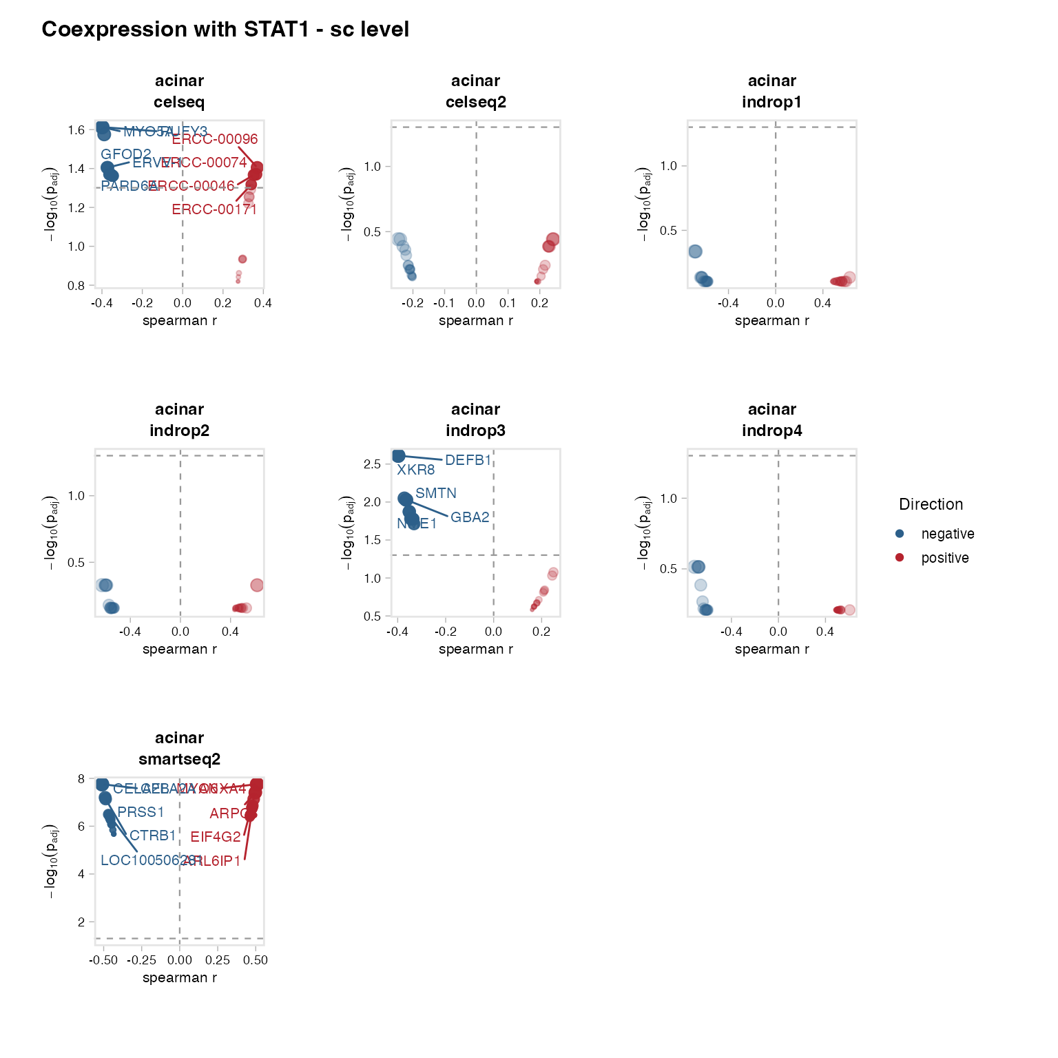
5. SplitByGene() - label cells for downstream
analysis
SplitByGene() adds a new metadata column splitting cells
into expression groups within each cell type. The column plugs straight
into RunGSEA_pseudobulk() (as contrast.by) or
Seurat::FindMarkers().
Default: zero vs. expressed
panc8 <- SplitByGene(panc8,
  gene     = "STAT1",
  group.by = "celltype",
  split    = "zero_vs_expressed")
## celltype
## STAT1_split acinar activated_stellate alpha beta delta ductal endothelial
## expressed 772 227 2209 1393 359 1065 43
## zero 1092 247 2406 2286 654 889 253
## celltype
## STAT1_split epsilon gamma macrophage mast quiescent_stellate schwann
## expressed 15 306 44 11 36 8
## zero 15 319 35 45 144 17
# New column "STAT1_split" is now in meta.data:
table(panc8$STAT1_split, panc8$celltype, useNA = "ifany")
##
## acinar activated_stellate alpha beta delta ductal endothelial
## expressed 772 227 2209 1393 359 1065 43
## zero 1092 247 2406 2286 654 889 253
##
## epsilon gamma macrophage mast quiescent_stellate schwann
## expressed 15 306 44 11 36 8
## zero 15 319 35 45 144 17Quantile split
panc8 <- SplitByGene(panc8,
  gene           = "STAT1",
  group.by       = "celltype",
  split          = "quantile",
  quantile_range = c(0.25, 0.75))  # bottom 25% = "low", top 25% = "high"
Middle cells (between the two quantiles) receive NA and
are excluded from downstream tests, keeping only the contrast
extremes.
Feeding into RunGSEA_pseudobulk()
RunGSEA_pseudobulk(panc8,
  group.by    = "celltype",
  sample.by   = "donor",
  contrast.by = "STAT1_split",
  pathway_sets = list( Hallmark = list(category = "H")),
  species     = "human",
  output_dir  = "./Figures/STAT1_pseudobulk_GSEA")
Feeding into RunWilcoxAUC()
markers <- RunWilcoxAUC(panc8,
  group.by  = "STAT1_split",split.by="celltype",
  min.pct   = 0.1,
  logfc.threshold = 0.25)
head(markers)
## celltype feature group avgExpr logFC statistic auc
## 1 gamma A1BG-AS1 expressed 0.0086168257 0.0073175175 50598.5 0.5183529
## 2 gamma A1BG expressed 0.2699636005 0.1362715557 62992.0 0.6453173
## 3 gamma A1CF expressed 0.5195332278 0.1377585800 59419.0 0.6087139
## 4 gamma A2M-AS1 expressed 0.0139130153 0.0067855068 50098.0 0.5132256
## 5 gamma A2ML1 expressed 0.0052403089 -0.0005868226 50115.0 0.5133997
## 6 gamma A2MP1 expressed 0.0001736141 0.0001736141 48966.5 0.5016340
## pval padj pct_in pct_out
## 1 7.617306e-03 2.366026e-02 4.9019608 1.253918
## 2 1.376288e-13 1.060389e-11 50.3267974 19.749216
## 3 4.934176e-07 4.048545e-06 64.3790850 36.050157
## 4 3.659151e-02 9.559750e-02 3.9215686 1.253918
## 5 5.738417e-02 1.394056e-01 4.5751634 1.880878
## 6 3.087634e-01 5.437977e-01 0.3267974 0.000000See also
- Vignette 05:
GroupHeatmap(),SplitDotPlot()- expression summaries per cell type - Vignette 08:
RunGSEA()- pathway analysis on a gene list - Vignette 09:
RunGSEA_pseudobulk()- full pseudobulk GSEA pipeline (contrast.byaccepts the column fromSplitByGene)
Session info
## R version 4.3.1 (2023-06-16)
## Platform: aarch64-apple-darwin20 (64-bit)
## Running under: macOS 15.6
##
## Matrix products: default
## BLAS:   /Library/Frameworks/R.framework/Versions/4.3-arm64/Resources/lib/libRblas.0.dylib
## LAPACK: /Library/Frameworks/R.framework/Versions/4.3-arm64/Resources/lib/libRlapack.dylib;  LAPACK version 3.11.0
##
## locale:
## [1] en_US.UTF-8/en_US.UTF-8/en_US.UTF-8/C/en_US.UTF-8/en_US.UTF-8
##
## time zone: America/Chicago
## tzcode source: internal
##
## attached base packages:
## [1] stats     graphics  grDevices utils     datasets  methods   base
##
## other attached packages:
##  [1] stxBrain.SeuratData_0.1.2 pbmc3k.SeuratData_3.1.4
##  [3] panc8.SeuratData_3.0.2    ifnb.SeuratData_3.1.0
##  [5] bmcite.SeuratData_0.3.0   SeuratData_0.2.2
##  [7] Seurat_5.2.1              SeuratObject_5.1.0
##  [9] sp_2.1-3                  scSidekick_1.2.0
##
## loaded via a namespace (and not attached):
##   [1] RColorBrewer_1.1-3     rstudioapi_0.16.0      jsonlite_2.0.0
##   [4] magrittr_2.0.3         spatstat.utils_3.1-0   farver_2.1.2
##   [7] rmarkdown_2.29         fs_1.6.6               ragg_1.4.0
##  [10] vctrs_0.6.5            ROCR_1.0-11            spatstat.explore_3.2-7
##  [13] htmltools_0.5.8.1      sass_0.4.10            sctransform_0.4.1
##  [16] parallelly_1.37.1      KernSmooth_2.23-22     bslib_0.9.0
##  [19] htmlwidgets_1.6.4      desc_1.4.3             ica_1.0-3
##  [22] plyr_1.8.9             plotly_4.10.4          zoo_1.8-14
##  [25] cachem_1.1.0           igraph_2.0.3           mime_0.13
##  [28] lifecycle_1.0.4        pkgconfig_2.0.3        Matrix_1.6-5
##  [31] R6_2.6.1               fastmap_1.2.0          fitdistrplus_1.1-11
##  [34] future_1.33.2          shiny_1.11.1           digest_0.6.37
##  [37] colorspace_2.1-1       patchwork_1.3.1        tensor_1.5
##  [40] RSpectra_0.16-1        irlba_2.3.5.1          textshaping_0.3.7
##  [43] labeling_0.4.3         progressr_0.14.0       spatstat.sparse_3.0-3
##  [46] httr_1.4.7             polyclip_1.10-6        abind_1.4-8
##  [49] compiler_4.3.1         withr_3.0.2            S7_0.2.0
##  [52] fastDummies_1.7.3      highr_0.10             MASS_7.3-60.0.1
##  [55] rappdirs_0.3.3         tools_4.3.1            lmtest_0.9-40
##  [58] otel_0.2.0             httpuv_1.6.16          future.apply_1.11.2
##  [61] goftest_1.2-3          glue_1.8.0             nlme_3.1-164
##  [64] promises_1.5.0         grid_4.3.1             Rtsne_0.17
##  [67] cluster_2.1.6          reshape2_1.4.4         generics_0.1.4
##  [70] gtable_0.3.6           spatstat.data_3.0-4    tidyr_1.3.1
##  [73] data.table_1.15.4      spatstat.geom_3.2-9    RcppAnnoy_0.0.22
##  [76] ggrepel_0.9.6          RANN_2.6.1             pillar_1.11.0
##  [79] stringr_1.5.1          limma_3.58.1           spam_2.10-0
##  [82] RcppHNSW_0.6.0         later_1.4.2            splines_4.3.1
##  [85] dplyr_1.1.4            lattice_0.22-6         survival_3.5-8
##  [88] deldir_2.0-4           tidyselect_1.2.1       locfit_1.5-9.9
##  [91] miniUI_0.1.1.1         pbapply_1.7-2          knitr_1.45
##  [94] gridExtra_2.3          edgeR_4.0.16           scattermore_1.2
##  [97] xfun_0.52              statmod_1.5.0          matrixStats_1.2.0
## [100] stringi_1.8.7          lazyeval_0.2.2         yaml_2.3.10
## [103] evaluate_0.23          codetools_0.2-20       tibble_3.3.0
## [106] cli_3.6.5              uwot_0.1.16            xtable_1.8-4
## [109] reticulate_1.42.0      systemfonts_1.3.2      jquerylib_0.1.4
## [112] dichromat_2.0-0.1      Rcpp_1.1.0             globals_0.16.3
## [115] spatstat.random_3.2-3  png_0.1-8              parallel_4.3.1
## [118] pkgdown_2.1.3          ggplot2_4.0.3          presto_1.0.0
## [121] dotCall64_1.1-1        listenv_0.9.1          viridisLite_0.4.2
## [124] scales_1.4.0           ggridges_0.5.6         purrr_1.0.4
## [127] crayon_1.5.2           rlang_1.1.6            cowplot_1.2.0.9000