
scSidekick - Large Datasets: BPCells, Sketch, Pseudobulk & Clinical Metadata
14_large_data.RmdOverview
Atlas-scale objects (hundreds of thousands to millions of cells) break the usual “load everything into memory” assumption. scSidekick is built to scale in two complementary ways:
-
Streaming heavy functions - feature plots,
pseudobulk aggregation, and pathway scoring read BPCells / on-disk and
Sketchassays lazily. Only the genes (or cells) you ask for are pulled off disk, so the same one-liners run on a 2-million-cell object without materialising it. - Aggregating to a tractable unit - collapse millions of cells to per-sample pseudobulk profiles, then analyze those with fast, robust, sample-level statistics.
1. BPCells & on-disk assays
With a BPCells-backed object the count matrix lives on disk, not in RAM. scSidekick’s plotting and aggregation functions detect the lazy matrix and stream through it - they subset the requested rows before materialising, so memory stays flat regardless of object size.
library(BPCells)

# Write a 10x matrix to a BPCells on-disk directory (once):
mat <- open_matrix_10x_hdf5("filtered_feature_bc_matrix.h5")
write_matrix_dir(mat, dir = "bp_counts")

# Build a Seurat object whose counts are the on-disk matrix:
counts <- open_matrix_dir("bp_counts")
obj    <- CreateSeuratObject(counts) |>
  NormalizeData() |>
  FindVariableFeatures() |>
  ScaleData() |>
  RunPCA() |>
  RunUMAP(dims = 1:30)

obj <- PrepObject(obj,
  variables  = c("Sample", "Group", "seurat_clusters"),
  group.by   = "seurat_clusters",
  output_dir = "./Figures")

# These behave exactly as on an in-memory object - but only the requested
# genes are read off disk for each panel:
PlotFeaturePlots(obj, features = c("CD3E", "LYZ", "NKG7"), split.by = "Sample")
GroupHeatmap(obj, features = marker_genes)
2. The Sketch workflow
For interactive work on millions of cells, Seurat v5’s
SketchData() keeps a representative subset “in memory”
while the full data stays on disk. scSidekick functions work on either
assay - sketch for fast iteration, full for the final figure.
obj <- SketchData(obj, ncells = 50000, method = "LeverageScore",
                  sketched.assay = "sketch")

# Iterate fast on the sketch assay ...
DefaultAssay(obj) <- "sketch"
PlotFeaturePlots(obj, features = "CD3E", split.by = "Sample")

# ... then project back to the full dataset for the publication figure.
# (For pseudobulk / pathway analysis on sketched objects, pass assay = "RNA"
#  explicitly so aggregation uses the full data, not the sketch.)
3. Pseudobulk: collapse cells to samples
Pseudobulk is the most robust way to analyze large multi-sample
studies: sum (or average) each gene within each sample, then treat
samples as replicates. ComputePseudobulk() streams the
matrix once (BPCells-safe) and caches the result in the object;
PlotPseudoBulk() draws per-gene, per-group profiles with
one point per donor.
bmcite <- ComputePseudobulk(bmcite,
  group.by = c("donor", "celltype.l1"),
  genes    = c("LYZ", "CD3D", "NKG7", "CD79A", "S100A8"),
  verbose  = FALSE)
PlotPseudoBulk(bmcite,
  features = c("LYZ", "CD3D"),
  group.by = "celltype.l1",
  donor.by = "donor")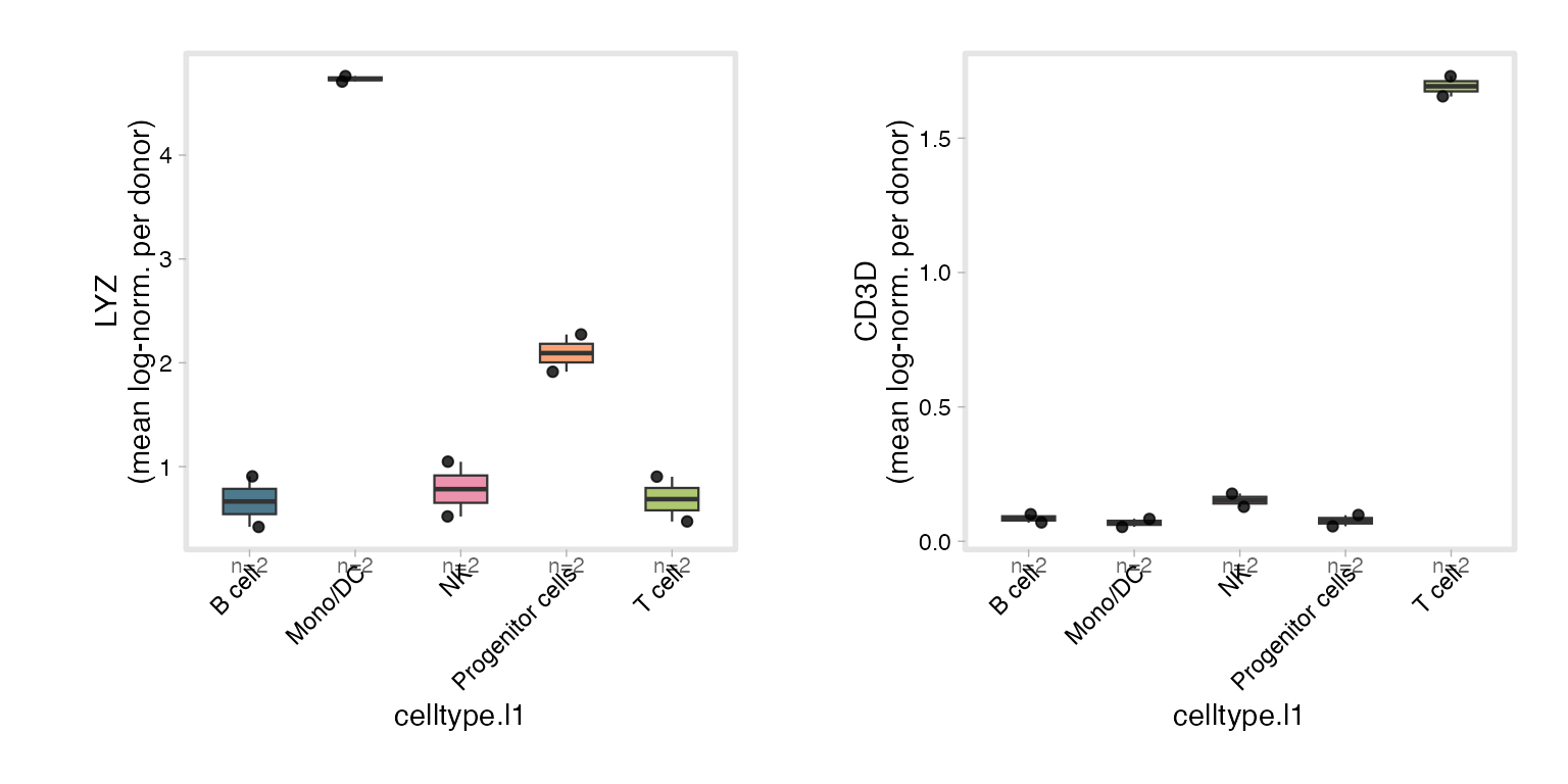
With more samples you can add cross-group statistics directly:
PlotPseudoBulk(obj,
  features    = "APOE",
  group.by = "Cognitive.Status",
  donor.by = "Donor.ID",
  split.by = "CellType",
  exclude     = list(Cognitive.Status = "Reference"),
  add_stats   = TRUE,
  ref_group   = "No dementia",
  min_cells   = 10)
4. Adding clinical metadata - AddClinicalMeta()
Large cohort studies always ship with a separate clinical table (age,
disease status, treatment arm, etc.) keyed by donor or sample ID.
AddClinicalMeta() joins that table onto every cell in one
call, matching on any column in meta.data - no manual
match() loops needed.
# Build a small illustrative clinical table from bmcite's actual donor IDs
donors   <- unique(bmcite$donor)
clinical <- data.frame(
  DonorID    = donors,
  Age        = c(34L, 27L, 45L, 52L, 38L, 61L, 29L, 47L)[seq_along(donors)],
  Disease    = rep_len(c("AML", "Normal"), length(donors)),
  stringsAsFactors = FALSE
)

# One call broadcasts each donor's clinical data to all its cells
bmcite <- AddClinicalMeta(bmcite, clinical,
                          by     = "donor",
                          df.key = "DonorID")

head(bmcite[[c("donor", "Age", "Disease")]], 4)
## donor Age Disease
## a_AAACCTGAGCTTATCG-1 batch1 34 AML
## a_AAACCTGAGGTGGGTT-1 batch1 34 AML
## a_AAACCTGAGTACATGA-1 batch1 34 AML
## a_AAACCTGCAAACCTAC-1 batch1 34 AMLThe columns argument lets you pick specific fields, and
prefix namespaces them if you are joining multiple
tables:
# Join only selected columns
obj <- AddClinicalMeta(obj, clinical,
                       by      = "donor.id",
                       df.key  = "PatientID",
                       columns = c("Age", "IDH_status", "Grade"))

# Join a second table with a prefix to avoid name collisions
obj <- AddClinicalMeta(obj, imaging,
                       by      = "donor.id",
                       df.key  = "PatientID",
                       prefix  = "mri.")
Once the columns are on the object you can use them anywhere -
split.by, group.by, facet_col in
survival plots, or as covariates in pseudobulk DE.
5. Pathway analysis at scale
Two routes, both designed for big objects:
Donor-level GSEA - RunGSEA_pseudobulk()
Pseudobulk -> per-contrast differential expression -> GSEA against Hallmark / KEGG / Reactome / WikiPathways, plus optional ssGSEA. Sample-level statistics mean the result isn’t inflated by cell count.
RunGSEA_pseudobulk(obj,
  group.by    = "CellType",
  sample.by   = "Donor.ID",
  contrast.by = "Cognitive.Status",
  contrasts   = list(Dementia_vs_Control = "Dementia - No dementia"),
  species     = "human",
  output_dir  = "./Figures/Pathways_pseudobulk")
Per-cell ssGSEA - RunSCssGSEA()
When you want a pathway score per cell (e.g. to overlay on
the UMAP), RunSCssGSEA() computes single-cell ssGSEA and is
BPCells/sketch-aware (use assay = "RNA" /
"sketch" as appropriate).
RunSCssGSEA(obj,
  group.by         = "CellType",
  gene_set_library = "H",          # MSigDB Hallmark
  assay            = "sketch",     # score the sketch-subsampled assay instead of full "RNA"
  output_dir       = "./Figures/ssGSEA")
Tips for big objects
- Keep counts on disk with BPCells; scSidekick streams them.
- Use a sketch assay for interactive iteration, the
full assay for final figures - and pass
assay = "RNA"explicitly to pseudobulk/pathway functions so aggregation uses the full data. - Prefer pseudobulk (
ComputePseudobulk->PlotPseudoBulk,RunGSEA_pseudobulk) for differential and pathway analysis across samples - it’s both faster and statistically sounder than per-cell tests. - Use
AddClinicalMeta()to join sample-level covariates (age, disease, treatment) before any split or facet operation - the columns become available everywhere once they are on the object.
See also
- Vignette 08:
RunGSEA()- cell-level pathway analysis (keyword search, leading-edge visualization) - Vignette 09:
RunGSEA_pseudobulk()- full pseudobulk GSEA with limma-voom - Vignette 13:
PlotMetaSummary()- donor-level summaries for large cohorts - Vignette 04:
PlotFeaturePlots()- the streaming feature-map function
Session info
## R version 4.3.1 (2023-06-16)
## Platform: aarch64-apple-darwin20 (64-bit)
## Running under: macOS 15.6
##
## Matrix products: default
## BLAS:   /Library/Frameworks/R.framework/Versions/4.3-arm64/Resources/lib/libRblas.0.dylib
## LAPACK: /Library/Frameworks/R.framework/Versions/4.3-arm64/Resources/lib/libRlapack.dylib;  LAPACK version 3.11.0
##
## locale:
## [1] en_US.UTF-8/en_US.UTF-8/en_US.UTF-8/C/en_US.UTF-8/en_US.UTF-8
##
## time zone: America/Chicago
## tzcode source: internal
##
## attached base packages:
## [1] stats     graphics  grDevices utils     datasets  methods   base
##
## other attached packages:
##  [1] stxBrain.SeuratData_0.1.2 pbmc3k.SeuratData_3.1.4
##  [3] panc8.SeuratData_3.0.2    ifnb.SeuratData_3.1.0
##  [5] bmcite.SeuratData_0.3.0   SeuratData_0.2.2
##  [7] Seurat_5.2.1              SeuratObject_5.1.0
##  [9] sp_2.1-3                  scSidekick_1.2.0
##
## loaded via a namespace (and not attached):
##   [1] RColorBrewer_1.1-3     rstudioapi_0.16.0      jsonlite_2.0.0
##   [4] magrittr_2.0.3         spatstat.utils_3.1-0   farver_2.1.2
##   [7] rmarkdown_2.29         fs_1.6.6               ragg_1.4.0
##  [10] vctrs_0.6.5            ROCR_1.0-11            spatstat.explore_3.2-7
##  [13] htmltools_0.5.8.1      sass_0.4.10            sctransform_0.4.1
##  [16] parallelly_1.37.1      KernSmooth_2.23-22     bslib_0.9.0
##  [19] htmlwidgets_1.6.4      desc_1.4.3             ica_1.0-3
##  [22] plyr_1.8.9             plotly_4.10.4          zoo_1.8-14
##  [25] cachem_1.1.0           igraph_2.0.3           mime_0.13
##  [28] lifecycle_1.0.4        pkgconfig_2.0.3        Matrix_1.6-5
##  [31] R6_2.6.1               fastmap_1.2.0          fitdistrplus_1.1-11
##  [34] future_1.33.2          shiny_1.11.1           digest_0.6.37
##  [37] colorspace_2.1-1       patchwork_1.3.1        tensor_1.5
##  [40] RSpectra_0.16-1        irlba_2.3.5.1          textshaping_0.3.7
##  [43] labeling_0.4.3         progressr_0.14.0       spatstat.sparse_3.0-3
##  [46] httr_1.4.7             polyclip_1.10-6        abind_1.4-8
##  [49] compiler_4.3.1         withr_3.0.2            S7_0.2.0
##  [52] fastDummies_1.7.3      highr_0.10             MASS_7.3-60.0.1
##  [55] rappdirs_0.3.3         tools_4.3.1            lmtest_0.9-40
##  [58] otel_0.2.0             httpuv_1.6.16          future.apply_1.11.2
##  [61] goftest_1.2-3          glue_1.8.0             nlme_3.1-164
##  [64] promises_1.5.0         grid_4.3.1             Rtsne_0.17
##  [67] cluster_2.1.6          reshape2_1.4.4         generics_0.1.4
##  [70] gtable_0.3.6           spatstat.data_3.0-4    tidyr_1.3.1
##  [73] data.table_1.15.4      spatstat.geom_3.2-9    RcppAnnoy_0.0.22
##  [76] ggrepel_0.9.6          RANN_2.6.1             pillar_1.11.0
##  [79] stringr_1.5.1          spam_2.10-0            RcppHNSW_0.6.0
##  [82] later_1.4.2            splines_4.3.1          dplyr_1.1.4
##  [85] lattice_0.22-6         survival_3.5-8         deldir_2.0-4
##  [88] tidyselect_1.2.1       miniUI_0.1.1.1         pbapply_1.7-2
##  [91] knitr_1.45             gridExtra_2.3          scattermore_1.2
##  [94] xfun_0.52              matrixStats_1.2.0      stringi_1.8.7
##  [97] lazyeval_0.2.2         yaml_2.3.10            evaluate_0.23
## [100] codetools_0.2-20       tibble_3.3.0           cli_3.6.5
## [103] uwot_0.1.16            xtable_1.8-4           reticulate_1.42.0
## [106] systemfonts_1.3.2      jquerylib_0.1.4        dichromat_2.0-0.1
## [109] Rcpp_1.1.0             globals_0.16.3         spatstat.random_3.2-3
## [112] png_0.1-8              parallel_4.3.1         pkgdown_2.1.3
## [115] ggplot2_4.0.3          dotCall64_1.1-1        listenv_0.9.1
## [118] viridisLite_0.4.2      scales_1.4.0           ggridges_0.5.6
## [121] purrr_1.0.4            crayon_1.5.2           rlang_1.1.6
## [124] cowplot_1.2.0.9000